Linear Sweep Voltammetry/Cyclic Voltammetry

Introduction

Cyclic voltammetry (CV) is one of the most commonly used electrochemical techniques, and is based on a linear potential waveform; that is, the potential is changed as a linear function of time. The rate of change of potential with time is referred to as the scan rate.

The simplest technique that uses this waveform is Linear Sweep Voltammetry (LSV). The potential range is scanned starting at the Initial potential and ending at the Final potential. CV is an extension of LSV in that the direction of the potential scan is reversed at the end of the first scan (the first Switching Potential), and the potential range is scanned again in the reverse direction. The experiment can be stopped at the Final Potential, or the potential can be scanned past this potential to the second Switching Potential, where the direction of the potential scan is again reversed (Fig1). The potential can be cycled between the two Switching Potentials for several cycles before the experiment is ended at the Final Potential. Both LSV and CV are standard techniques on the epsilon. Multichannel CV experiments are also available through the addition of the optional bipotentiostat board.

Figure 1. Potential wave form for cyclic voltammetry.

Setting Up a Linear Sweep/Cyclic Voltammetry Experiment

The potential limits and the scan rate for LSV are set using the Change Parameters dialog box (Fig2) in either the Experiment menu or the pop-up menu.

Figure 2. Change Parameters dialog box for linear sweep voltammetry.

1. Potential values are entered in mV, and the Scan Rate in mV/s.
2. If the Apply Open Circuit Potential for Initial E box is checked, then the open circuit potential will automatically be measured and used as the Initial Potential.
3. If the Run - External Trigger box is checked, the experiment is started from an external device using the Start In back-panel connection.
4. When the experiment is started, the cell is held at the Initial Potential for the number of seconds defined by the Quiet Time.
5. The experiment can be run on a hanging mercury drop electrode (i.e., a single drop is used for the entire experiment) using a BASi® CGME by selecting CGME SMDE Mode from Cell Stand / Accessories in the Setup / Manual Settings (I/O) dialog box.
6. A rotating disk experiment can be run using a BASi® RDE-2 by selecting RDE-2 from Cell Stand / Accessories in the Setup / Manual Settings (I/O) dialog box and entering the required Rotation Rate under RDE2 Rotation in the Cell dialog box.
7. There are two gain stages for the current-to-voltage converter. The default values of these stages that are used for a given current Full Scale value are determined by the software. However, they can be adjusted manually using the Filter / F.S. dialog box. This dialog box is also used to change the analog Noise Filter Value settings from the default values set by the software.
8. The default condition of the cell is that the cell is On (i.e., the electronics are connected to the electrodes) during the experiment, and is Offbetween experiments. However, the potential can be switched Onbetween experiments using the Cell dialog box. HOWEVER, THIS OPTION SHOULD BE USED WITH CAUTION SINCE CONNECTING OR DISCONNECTING THE ELECTRODES WHEN THE CELL IS ON CAN RESULT IN DAMAGE TO THE POTENTIOSTAT, THE CELL, AND/OR THE USER!
9. A series of identical experiments on the same cell can be programmed using the MR (Multi-Run) option.
10. Clicking the IR-COMP button activates the iR compensation option.
11. Clicking Exit will exit the dialog box without saving any changes made to the parameter values. Any changes can be saved by clicking Apply before exiting.
12. Range of allowed parameter values:
    • Potential = -3275 - +3275 mV
    • Scan Rate = 1 - 25,000 mV/s (also see below for further discussion)
    • Quiet Time = 0 - 100 s
13. Once the parameters have been set, the experiment can be started by clicking Run (either in this dialog box, in the Experiment menu, in the pop-up menu, on the Tool Bar, or using the F5 key).

Up to four parameters are used in the epsilon software to define the potential wave form for CV.

1. Initial Potential
2. Switching Potential 1
3. Switching Potential 2
4. Final Potential

The defined waveform will also depend upon the number of segments.

• 1 segment - Initial Potential - Final Potential (this is equivalent to an LSV experiment)
• 2 segments - Initial Potential - Switching Potential 1 - Final Potential
• 3 segments - Initial Potential - Switching Potential 1 - Switching Potential 2 - Final Potential (setting Final Potential equal to Initial Potential will generate a complete potential cycle)
• 4 segments - Initial Potential - Switching Potential 1 - Switching Potential 2 - Switching Potential 1- Final Potential

The potential limits and the scan rate for CV are set using the Change Parameters dialog box (Fig3) in either the Experiment menu or the pop-up menu.

Figure 3. Change Parameters dialog box for cyclic voltammetry.

1. Potential values are entered in mV, and the Scan Rate in mV/s.
2. If the Apply Open Circuit Potential for Initial E box is checked, then the open circuit potential will automatically be measured and used as the Initial Potential.
3. If the Run - External Trigger box is checked, the experiment is started from an external device using the Start In back-panel connection.
4. When the experiment is started, the cell is held at the Initial Potential for the number of seconds defined by the Quiet Time.
5. The experiment can be run on a hanging mercury drop electrode (i.e., a single drop is used for the entire experiment) using a BASi® CGME by selecting CGME SMDE Mode from Cell Stand / Accessories in the Setup / Manual Settings (I/O) dialog box.
6. A rotating disk experiment can be run using a BASi® RDE-2 by selecting RDE-2 from Cell Stand / Accessories in the Setup / Manual Settings (I/O) dialog box and entering the required Rotation Rate under RDE2 Rotation in the Cell dialog box.
7. There are two gain stages for the current-to-voltage converter. The default values of these stages that are used for a given current Full Scale value are determined by the software. However, they can be adjusted manually using the Filter / F.S. dialog box. This dialog box is also used to change the analog Noise Filter Value settings from the default values set by the software.
8. The default condition of the cell is that the cell is On (i.e., the electronics are connected to the electrodes) during the experiment, and is Offbetween experiments. However, the potential can be switched Onbetween experiments using the Cell dialog box. HOWEVER, THIS OPTION SHOULD BE USED WITH CAUTION SINCE CONNECTING OR DISCONNECTING THE ELECTRODES WHEN THE CELL IS ON CAN RESULT IN DAMAGE TO THE POTENTIOSTAT, THE CELL, AND/OR THE USER!
9. A series of identical experiments on the same cell can be programmed using the MR (Multi-Run) option.
10. Clicking the IR-COMP button activates the iR compensation option.
11. Clicking Exit will exit the dialog box without saving any changes made to the parameter values. Any changes can be saved by clicking Apply before exiting.
12. Range of allowed parameter values:
    • Potential = -3275 - +3275 mV
    • Scan Rate = 1 - 25,000 mV/s (also see below)
    • Quiet Time = 0 - 100 s
    • The # of Segments is limited by the total number of data points that can be stored (64,000) (note that in this initial version, the potential resolution of the current measurement is fixed at 1 mV).
13. Once the parameters have been set, the experiment can be started by clicking Run (either in this dialog box, in the Experiment menu, in the pop-up menu, on the Tool Bar, or using the F5 key).

Scan Rates

The digital waveform generator approximates a linear waveform with a staircase waveform with 100 mV steps. Since the waveform is generated digitally (the digital-to-analog converter clock speed is 1 MHz), only discrete scan rates are allowed because the step time is obtained by dividing the clock speed by integer values. The allowable scan rates (shown T1) are given by the equation:

 

Scan Rate (mV/s) = 100,000/n, where n is an integer

Thus, if a scan rate is entered that does not match the allowed values, the software will automatically change it to the nearest allowed value. The maximum scan rate allowed is 10,000 mV/s due to hardware limitations.

n	Scan Rate/mV s-1	Approx. resolution/mV s-1
4	25,000
5	20,000
6	16,667
7	14,286
8	12,500
9	11,111
10	10,000
11	9,091
12	8,330
13	7,692
14	7,143
15	6,667
16	6,250
17	5,882
18	5,556
19	5,263
20	5,000
21-50	5,000-2,000	240
50-100	2,000-1,000	40
100-200	1,000-500	10
200-500	500-200	3
500-100,000	200-1	1

Analysis of the Current Response

The asymmetric shape of the current-voltage plot of a CV or an LSV experiment (a cyclic or linear sweep voltammogram, respectively) can be rationalized by considering the concentration profiles at different time points for O and R for the reduction reaction O + e^- = R (Fig4).

Figure 4. Concentration profiles for cyclic voltammetry for a simple reduction reaction. Simulation by DigiSim ^®.

At the start of the experiment, the bulk solution contains only O, so at potentials well positive of the redox potentials, there is no net conversion of O to R (a). As the redox potential is approached, there is a net cathodic current which increases exponentially with potential due to the exponential potential dependence of the rate of heterogeneous electron transfer. As O is converted to R, concentration gradients are set up for both O and R, and diffusion occurs down these gradients (O diffuses towards the electrode, and R diffuses in the opposite direction). The redox potential is at b, and the surface concentrations of O and R are equal at this potential. After the (cathodic) peak potential (c), the current decays as a result of the depletion of O in the interfacial region. The rate of electrolysis (and hence the current) now depends on the rate of mass transport of O from the bulk solution to the electrode surface; that is, it is dependent on the rate of diffusion of O, so the time dependence is t ^-½. The peak is therefore asymmetric. Upon reversal of the direction of the potential scan (in a CV experiment), the current continues to decay with t ^-½ until the potential nears the redox potential, at which point there begins a net reoxidation of R to O which causes an anodic current. However, some R molecules have diffused away from the electrode surface, and so have to diffuse back to the electrode before they can be reoxidized. Therefore, the current does not decay to zero following the reoxidation (anodic) peak on the reverse scan (h). The important parameters for a linear sweep (Fig5) or cyclic voltammogram (Fig6) are the peak potential(s) E_p and the peak current(s) i_p (note that there can be more than one peak in a cyclic voltammogram; hence an additional subscript (a = anodic, c = cathodic) is often used). The measurement of these parameters, and their significance, is discussed in more detail in a later section.

Figure 5. A typical linear sweep voltammogram showing the important parameters.

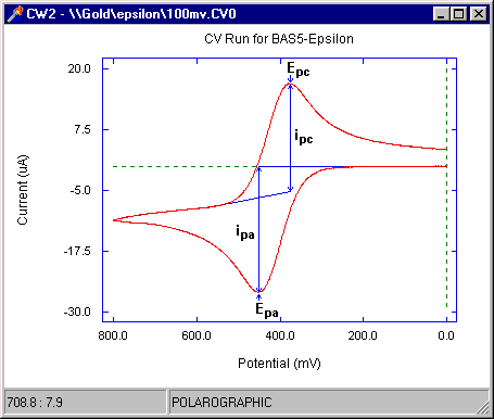
Figure 6. A typical cyclic voltammogram showing the important parameters.

Semidifferentation and Semiintegration

The default plot for LSV and CV is the current vs. potential plot. However, two other plots are available using Select - Graph in the pop-up menu - SemiIntegration (Fig7)and SemiDifferentiation (Fig8). These are mathematical transforms of the basic current vs. potential plot.

Figure 7. A typical cyclic voltammogram following semiintegration.

Figure 8. A typical cyclic voltammogram following semidifferentiation.

Display Selected Segments

Choosing Selected Segments in the Select Graph options allow one to view and print selected segments of the CV experiments. The dialog box (Fig9) will initially show all segments in the display list. One can move all segments out of Display list with the << button and move all into the Display list with the >> button. Highlighted individual and multiple segments can be to move out of the display list < or into the display list >. Once the desired segments are listed, then clicking the Redraw button will redraw the graph with only the selected segments shown. Two other options with the display are whether to Show Peaks (show the baseline and peak lines) and whether to Paint Peaks (show shading for area of peak).

Figure 9. Selected segments dialog box.

With the selected Segments Display, one can perform the following operations and the selected peaks will remain displayed.

• Smooth Data
• Change Display Type
• Grid
• Show Data Points
• Copy to Clip-Board
• Text Info
• Select Colors and Fonts
• Manual Zoom
• Zoom with mouse

Performing the following commands will reset the display to all segments.

• Raw Data
• Processed data
• Auto zoom (Processed Data)
• Zoom out (Processed Data)
• Peak finding (Processed Data)

If one goes from SemiDiff or SemiInt to Display Segment, the display resets to the normal Processed Data Display.

DigiSim is a registered trademark of Bioanalytical Systems, Inc.

---

Back to Table of Contents