Chronoamperometry/chronocoulometry

Introduction

Chronoamperometry (CA) and chronocoulometry (CC) have the same potential wave form - the potential step - which is one of the simplest potential wave forms. As shown below (Fig1), the potential is changed instantaneously from the Initial Potential to the First Step Potential, and it is held at this value for the First Step Time. This is a single potential step experiment. In a double potential step experiment, the potential is changed to the Second Step Potential after the First Step Time, and it is then held at this value for the Second Step Time. In CA, the current is monitored as a function of time, whereas in CC, the charge is monitored as a function of time. It is important to note that the basic potential step experiment on the epsilon is CA; that is, during the experiment, the current is recorded as a function of time. However, after the experiment, the data can also be displayed as charge as a function of time (the charge is calculated by integrating the current). Hence, chronocoulometry data can be obtained. CA is a standard technique on the epsilon.

CA is different from other constant potential techniques (constant potential electrolysis (CPE) and DC potential amperometry (DCA)) in that the time scale of CA is shorter (milliseconds and seconds) than those of CPE and DCA (seconds and minutes).

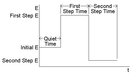
Figure 1. Potential wave form for chronoamperometry and chronocoulometry.

Setting Up a Chronoamperometry/Chronocoulometry Experiment

As shown above, five parameters are used in the epsilon software to define the potential wave form for CA.

1. Initial Potential
2. First Step Potential (E)
3. Second Step Potential (E)
4. First Step Time
5. Second Step Time

The values of these parameters are set using the Change Parameter dialog box (Fig2) in either the Experiment menu or the pop-up menu.

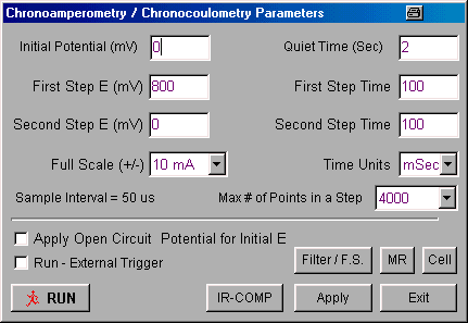
Figure 2. Change Parameters dialog box for chronoamperometry/chronocoulometry.

1. Potential values are entered in mV, and time values in ms or s (select using Time Units).
2. If the Apply Open Circuit Potential for Initial E box is checked, then the open circuit potential will automatically be measured and used as the Initial Potential.
3. If the Run - External Trigger box is checked, the experiment is started from an external device using the Start In back-panel connection.
4. When the experiment is started, the cell is held at the Initial Potential for the number of seconds defined by the Quiet Time.
5. The experiment can be run on a hanging mercury drop electrode (i.e., a single drop is used for the entire experiment) using a BASi® CGME by selecting CGME SMDE Mode from Cell Stand / Accessories in the Setup / Manual Settings (I/O) dialog box.
6. A rotating disk experiment can be run using a BASi® RDE-2 by selecting RDE-2 from Cell Stand / Accessories in the Setup / Manual Settings (I/O) dialog box and entering the required Rotation Rate under RDE2 Rotation in the Cell dialog box.
7. There are two gain stages for the current-to-voltage converter. The default values of these stages that are used for a given current Full Scale value are determined by the software. However, they can be adjusted manually using the Filter / F.S. dialog box. This dialog box is also used to change the analog Noise Filter Value settings from the default values set by the software.
8. The default condition of the cell is that the cell is On (i.e., the electronics are connected to the electrodes) during the experiment, and is Offbetween experiments. However, the potential can be switched Onbetween experiments using the Cell dialog box. HOWEVER, THIS OPTION SHOULD BE USED WITH CAUTION SINCE CONNECTING OR DISCONNECTING THE ELECTRODES WHEN THE CELL IS ON CAN RESULT IN DAMAGE TO THE POTENTIOSTAT, THE CELL, AND/OR THE USER!
9. A series of identical experiments on the same cell can be programmed using the MR (Multi-Run) option.
10. Clicking Exit will exit the dialog box without saving any changes made to the parameter values. Any changes can be saved by clicking Apply before exiting.
11. Range of allowed parameter values:
    • Potential = -3275 mV - +3275 mV
    • Quiet Time = 0 - 100 s
    • Step Time = 1 - 65 s OR 1 - 16000 ms
    • Maximum # of points in a step = 1000, 2000, 4000, 8000, 16000
    • The Sample Interval is determined by the Step Time and the Maximum # of points in a step, and can only be adjusted by the user indirectly through these latter two parameters. The relationship between these parameters is shown by the equation

      Sample Interval = Step Time/Maximum # of points

      However, it should be noted that only certain values are allowed for each of these parameters, as is shown in the table below:

      Max. # of points	1000	2000	4000	8000	16000
      Sample Interval	Maximum Step Time (/ms)
      20 ms	20	40	80	160	320
      50 ms	40	81	162	325	650
      100 ms	100	200	400	800	1600
      200 ms	200	400	800	1600	3200
      500 ms	406	812	1625	3250	6500
      1 ms	1000	2000	4000	8000	16000
      2 ms	2000	4000	8000	16000
      5 ms	4062	8125
      10 ms	10000

12. Once the parameters have been set, the experiment can be started by clicking Run (either in this dialog box, in the Experiment menu, in the pop-up menu, on the Tool Bar, or using the F5 key).

Analysis of the Current Response

Let us consider the effect of a single potential step on the reaction R = O + e^-. At potentials well negative of the redox potential (E_nr), there is no net conversion of R to O, whereas at potentials well positive of the redox potential (E_d), the rate of the reaction is diffusion-controlled (i.e., molecules of R are electrolyzed as soon as they arrive at the electrode surface). In most potential step experiments, E_nr is the Initial Potential, and E_d is the First Step Potential. The advantage of using these two potentials is that any effects of slow heterogeneous electron transfer kinetics are eliminated. In double potential step experiments, (E_nr) is often used as the Second Step Potential.

Figure 3. Concentration profiles for a single potential step experiment.

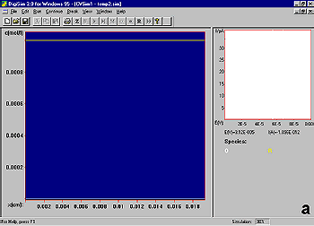
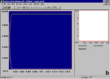
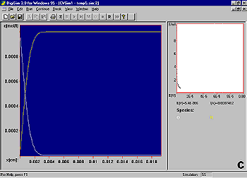
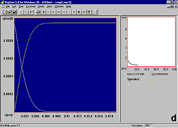
It is instructive to consider the concentration profiles of O and R following the potential step (Fig3). Initially, only R is present in solution (a). After the potential step, the concentration of R at the electrode surface decreases to zero, and hence a concentration gradient is set up between the interfacial region and the bulk solution (b). As molecules of R diffuse down this concentration gradient to the electrode surface (and are converted to O), a diffusion layer (i.e., a region of the solution in which the concentration of R has been depleted) is formed. The width of this layer increases with increasing time (b-d). There is also a net diffusion of O molecules away from the electrode surface.

Since the current is directly proportional to the rate of electrolysis, the current response to a potential step is a current 'spike' (due to initial electrolysis of species at the electrode surface) followed by time-dependent decay (Fig4) (due to diffusion of molecules to the electrode surface).

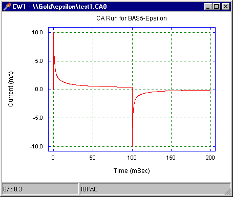
Figure 4. Current-time response for a double-potential step chronoamperometry experiment.

For a diffusion-controlled current, the current-time (i-t) curve is described by the Cottrell equation:

i = nFACD^½p^-½t ^-½

where:

n = number of electrons transferred/molecule F = Faraday's constant (96,500 C mol-1) A = electrode area (cm2) D = diffusion coefficient (cm2 s-1) C = concentration (mol cm-3)

The charge-time (Q-t) (the Anson equation) is obtained by integrating the Cottrell equation with respect to time, and can be displayed in the epsilon software by selecting Q vs T from Select Graph in the pop-up menu (the original i vs. t plot can be recovered by selecting Original from Select Graph in the pop-up menu). A typical charge-time plot is shown in Fig5:

Q = 2nFACD^½p^-½t ^½

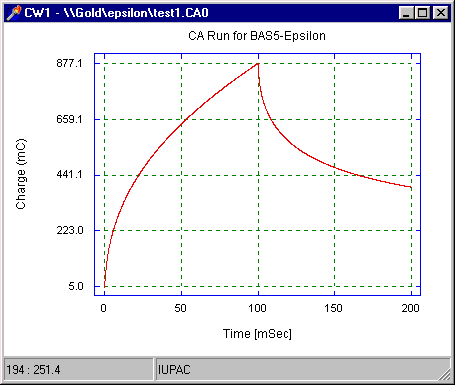
Figure 5. Charge-time response for a double-potential step chronocoulometry/chronoamperometry experiment.

Charge is the integral of current, so the response for CC increases with time, whereas that for CA decreases. Since the latter parts of the signal response must be used for data analysis (the finite rise time of the potentiostat invalidates the early time points), the larger signal response at the latter parts for CC makes this the more favorable potential step technique for many applications (in addition, integration decreases the noise level).

The analysis of CA and CC data is discussed elsewhere.

---

Back to Table of Contents